Anticipando il risultato a cui si giunge a fine sezione, si ottiene
e quindi
La trasformata di una costante è un impulso di area pari a valore della costante.L'analisi di questo caso consente di illustrare come l'impulso
Trattiamo
x![]() t
t![]() come un segnale periodico di periodo T
tendente ad
come un segnale periodico di periodo T
tendente ad ![]() 3.7, ed esprimiamolo nei termini dei coefficienti di Fourier: l'integrale
Xn =
3.7, ed esprimiamolo nei termini dei coefficienti di Fourier: l'integrale
Xn = ![]()
![]() A e-j2
A e-j2![]() nFtdt
per
T
nFtdt
per
T ![]()
![]() fornisce zero per tutti gli n tranne
che per n = 0, e quindi si ottiene Xn = A se n = 0, mentre
Xn = 0 se n
fornisce zero per tutti gli n tranne
che per n = 0, e quindi si ottiene Xn = A se n = 0, mentre
Xn = 0 se n ![]() 0.
0.
In alternativa, pensiamo la costante come il limite a cui tende un'onda quadra
con duty-cycle
![]() al tendere di
al tendere di ![]() a T:
lo spettro di ampiezza è stato calcolato al Capitolo 2, e presenta righe alle
armoniche
a T:
lo spettro di ampiezza è stato calcolato al Capitolo 2, e presenta righe alle
armoniche
![]() , mentre l'inviluppo di tipo
, mentre l'inviluppo di tipo
![]() si azzera alle frequenze
si azzera alle frequenze
![]() . Se
. Se
![]()
![]() T,
gli zeri annullano tutte le armoniche tranne X0, il cui valore
A
T,
gli zeri annullano tutte le armoniche tranne X0, il cui valore
A![]() tende ora ad A.
tende ora ad A.
Qualora invece si desideri calcolare la trasformata di Fourier anziché
la serie, applicando la definizione
X![]() f
f![]() =
= ![]() Ae-j2
Ae-j2![]() ftdt
si ottiene
X
ftdt
si ottiene
X![]() f
f![]() = 0 ovunque, tranne che in f = 0 dove
X
= 0 ovunque, tranne che in f = 0 dove
X![]() 0
0![]() =
= ![]() .
.
Notiamo ora che l'energia di
x![]()
![]() t
t![]() = Arect
= Arect![]()
![]() t
t![]() vale
vale
![]() x
x![]() =
= ![]()
![]() x
x![]()
![]() t
t![]()
![]() dt = A2
dt = A2![]() ;
per il teorema di Parseval, l'energia coincide nei dominii di tempo e frequenza,
e quindi risulta
;
per il teorema di Parseval, l'energia coincide nei dominii di tempo e frequenza,
e quindi risulta
 df = A2
 . Il formalismo dell'impulso matematico rende quindi possibile trattare il caso
in oggetto, in cui la potenza (finita) è tutta concentrata in un unico punto
(f = 0) dando luogo ad una densità infinita.
. Il formalismo dell'impulso matematico rende quindi possibile trattare il caso
in oggetto, in cui la potenza (finita) è tutta concentrata in un unico punto
(f = 0) dando luogo ad una densità infinita.
Resta da dimostrare quanto anticipato ad inizio sezione, ossia che
![]()
![]() A
A![]() = A
= A![]()
![]() f
f![]() .
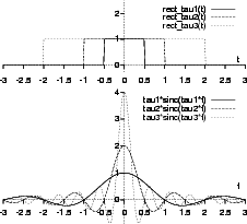
Abbiamo visto come
.
Abbiamo visto come
![]()
![]() Arect
Arect![]()
![]() t
t![]()
![]() = A
= A![]() sinc
sinc![]() f
f![]()
![]() ,
che per
,
che per
![]()
![]()
![]() vale
vale ![]() con f = 0 e
zero con f
con f = 0 e
zero con f ![]() 0. Ci troviamo quindi nelle esatte circostanze che definiscono
un impulso matematico, e resta da verificare che
0. Ci troviamo quindi nelle esatte circostanze che definiscono
un impulso matematico, e resta da verificare che
![]()
![]() sinc
sinc![]() f
f![]()
![]() df = 1:
si può mostrare (pag.
df = 1:
si può mostrare (pag. ![[*]](cross_ref_motif.gif) ) che l'integrale vale uno per
qualunque
) che l'integrale vale uno per
qualunque ![]() , e quindi possiamo scrivere
, e quindi possiamo scrivere
![]()
![]() A
A![]() = A .
= A . ![]()
![]() f
f![]() .
.